Physical Graph
The Physical Graph describes the topology in an abstract way and how the processing of the join happens. It can be either be created manually or be the result of an optimization process. A Physical Graph can then be transformed into a Storm Topology which can be run.
The Physical Graph is a directed graph with a bunch of labels. E.g., the following graph corresponds to the join between relations R and S:
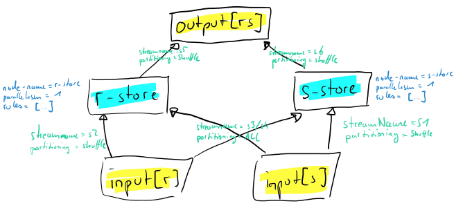
Here we see the yellow stub-nodes that represent sources of data (e.g., the stream named r originates from node input[r]) and sinks where results are sent to (e.g., the stream named rs is produced at all nodes that have edges towards output[rs]).
The blue nodes, here r-store and s-store are the locations where prefixes are stored. They are labeled with
- a node name for nicer identification of that component,
- a degree of parallelism that indicates the number of instances that are running that store in parallel, and
- a list of rules that determine the behaviour of that component, see below.
The nodes in the graph are connected via directed edges which are labelled with
- a stream name for nicer identification of the individual stream and
- a partitioning method that indicates, how messages should be distributed to the instances of each component, see below.
Rules
The nodes are labelled with rules. These rules specify a multitude of behaviours, e.g., if a tuple from stream s1 arrives, join it with stored tuples and send the result to stream s2.
Currently, there are these rules available:
IntermediateJoinRule: if a tuple arrives at the streamincomingStreamName, then join it usingpredicatesand send emerging results to streamoutgoingStreamName.JoinResultRule: if a tuple arrives at the streamincomingStreamName, then join it usingpredicatesand use emerging results as tuples forrelationName.StreamSendRule: if a new tuple forrelationNameis produced, send it to streamoutgoingStreamName
Partitioning Methods
Similar to Storm, in this Physical graph each node represents potentially multiple running instances and the edges between the nodes indicate communication flow. This means, we have to indicate, which message is sent to which instance of the component represented by a node.
This is specified by the partitioning method of the edge labels. The following partitioning methods are currently supported:
- shuffle: send it to any instance, round robin
- all: send it to all instances, broadcast
Implementation Notes
The physical graph lives in package de.unikl.dbis.clash.physical. The wrapper class to the internal components is the PhysicalGraph. It provides access to the internal nodes, connecting edges, and registered rules.